The pseudoclassical instantiation pattern is used in JavaScript to create objects with access to the same set of properties and methods. Unlike most programming languages, such as Java or C++, JavaScript does not have classes of objects. However, class-like objects can be created in JavaScript using several different instantiation patterns. The pseudoclassical pattern is the most widely used, because it takes advantage of prototypal inheritance.
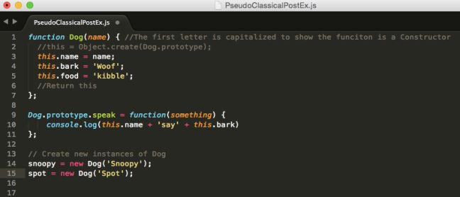
Prototypal inheritance is the ability of an object to delegate a property or method look-up to a parent object. In JavaScript, if an object does not have a particular method, a lookup is automatically performed on the object’s prototype (parent-like object). If the lookup is successful the method is passed along, and used as though the original object itself contained the method. Consider the following code:
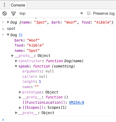
The Snoopy and Spot objects are created as new instances of the “Dog” prototype on lines 14 and 15 with the keyword “new”. This keyword is syntactic sugar that can be thought of as secretly inserting the commented text on lines 2 and 6. As a result, both snoopy and spot inherit all of the properties contained in the Dog constructor function as well as the speak method that belongs to the Dog prototype (this can be verified in the browser console).
By taking advantage of prototypal inheritance, the pseudoclassical pattern removes the need for functions to be repeatedly written and stored within multiple objects. This is why it is the most widely used constructor pattern for instantiating new objects in JavaScript.
Your Arduino project, using the Mega 2560, came out great and now you want to make a small production run as inexpensively as possible. Congratulations! That likely means you have successfully invented something you believe will be useful to others. This is an important step in your product’s development. You’ll need to pare down your project to include only essential components, and then test it before ordering custom PCBs. This post aims to help you in completing that task. It presents two methods that will enable you to isolate and program the atmega 2560 chip using the Arduino IDE. The presentation consists of step-by-step instructions for creating the required circuits, installing the Arduino bootloader, and installing a test sketch to ensure the chip is accepting and executing the uploaded programs. This post is intended for hobbyist inventors; however, professional electronic packaging engineers who are new to working the atmega 2560 may also benefit from reading it.
The first method is based on soldering an atmega 2560 to a TQFP100 package PCB (see figure on the right). For those hobbyists who are new to electronics packaging and circuit board design, the term “TQFP100 package” is a term that denotes a category of chips with specific dimensions. The atmega 2560 is one of many chips with these dimensions. This method is the least expensive way to isolate and program the chip with the Arduino IDE, so that your can test your prototype’s circuitry and make improvements. It is best suited for those who plan on doing very small production runs (i.e. less than 5 units). The method can also be used to salvage an atmega 2560 from an Arduino board that has failed in another area (i.e. USB serial adapter).
The second method is based on using a Yamaichi IC Test Socket & Programming Adapter for the TQFP100 package (see figure on right). This device allows a user to set up a circuit that can be used for rapidly programming a chip. It is a faster method for programming multiple chips, and a good option for production runs that do not warrant the expense of automating the chip programming process with robotics. The main drawback of the method is that it’s more expensive, and it is slightly more cumbersome for testing with breadboarded circuitry.
Method 1
This method is based on “breaking out” the atmega 2560 by soldering it to a PCB with DIP headers. In order to do that, and form the required circuitry, you will need the following parts:
An atmega 2560 chip
TQFP100 package (0.5 mm pitch) to DIP PCB
Female headers with .1” spacing
A soldering iron
.015 solder
Solder wick
A 10X loupe magnifier
Tape
Helping hands soldering aid (optional)
A multimeter
Breadboard
Jumper wires
Flux
16 MHz crystal
A 10 kΩ ¼ watt resistor
A 200Ω to 400Ω resistor
Two 22 pF ceramic capacitors
1 uF capacitor
A freetronics USB Serial Adaptor (with the included micro USB cable)
An Arduino Mega 2560 (with the required USB cable)
Begin building the circuit by soldering the atmega and headers to the PCB (see figure below). It is easiest to solder the chip if you begin by taping it to the PCB. Make sure that you orient the chip correctly before soldering it so that the numbers on the PCB correspond to the correct pins on the chip. If you are new to soldering Surface Mount Components, or have difficulty with soldering them you may want to watch this nice brief tutorial
You now have an atmega 2560 breakout board with which to create a circuit to upload the Arduino bootloader. The bootloader can be thought of as the chip’s operating system. It is the software that allows the chip to understand and use programs uploaded with the Arduino IDE. The bootloader program was created by Nick Gammon and can be downloaded from his website at http://www.gammon.com.au/bootloader. Use jumper wires to connect your Arduino Mega to the atmega breakout board with the following PIN assignments:
Arduino Mega pin D10 to Reset on atmega pin 30
Arduino Mega pin D51 to MOSI on atmega pin 21
Arduino Mega pin D50 for MISO on atmega pin 22
Arduino Mega pin D52 for SCK on atmega pin 20
Arduino Mega pin Gnd for Gnd on atmega pin 32
Arduino Mega pin +5V for +5V on atmega pin 31
Connect the 16.000 MHz Crystal to the atmega, via a breadboard, with the left leg of the crystal connected to XTAL2 (at pin 33 on the atmega) and the right leg of the crystal connected to XTAL1 (at pin 34 on the atmega).
The pin assignments for the atmega 2560 and Arduino Mega are illustrated in the figure above. You should now have a circuit that looks like the one depicted in the figure below.
Now upload the bootloader sketch and wait to see the following inside the serial monitor:
Atmega chip programmer.
Written by Nick Gammon.
Entered programming mode OK.
Signature = 0x1E 0x98 0x01
Processor = ATmega2560
Flash memory size = 262144 bytes.
LFuse = 0xFF
HFuse = 0xD8
EFuse = 0xFD
Lock byte = 0xCF
Bootloader address = 0x3E000
Bootloader length = 8192 bytes.
Type ‘G’ to program the chip with the bootloader …
Once you see the above, type “G” into the serial monitor to commence programming. You should see the following in the serial monitor:
Erasing chip …
Writing bootloader …
Committing page starting at 0x3E000
Committing page starting at 0x3E100
Committing page starting at 0x3E200
Committing page starting at 0x3E300
Committing page starting at 0x3E400
Committing page starting at 0x3E500
Committing page starting at 0x3E600
Committing page starting at 0x3E700
Committing page starting at 0x3E800
Committing page starting at 0x3E900
Committing page starting at 0x3EA00
Committing page starting at 0x3EB00
Committing page starting at 0x3EC00
Committing page starting at 0x3ED00
Committing page starting at 0x3EE00
Committing page starting at 0x3EF00
Committing page starting at 0x3F000
Committing page starting at 0x3F100
Committing page starting at 0x3F200
Committing page starting at 0x3F300
Committing page starting at 0x3F400
Committing page starting at 0x3F500
Committing page starting at 0x3F600
Committing page starting at 0x3F700
Committing page starting at 0x3F800
Committing page starting at 0x3F900
Committing page starting at 0x3FA00
Committing page starting at 0x3FB00
Committing page starting at 0x3FC00
Committing page starting at 0x3FD00
Committing page starting at 0x3FE00
Committing page starting at 0x3FF00
Written.
Verifying …
No errors found.
Writing fuses …
LFuse = 0xFF
HFuse = 0xD8
EFuse = 0xFD
Lock byte = 0xCF
Done.
Type ‘C’ when ready to continue with another chip …
With the bootloader installed you can start building the circuit for a test program (see figure on right). In this circuit the Freetronics USB Serial Adapter (FUSA) takes the place of the Arduino Mega from the previous circuit, and transfers the program from the Arduino IDE to the atmega 2560. Be sure to use the freetronics brand and not some other like FTDI, because they will not work. Freetronics uses Atmel’s ATmega16u2, which is essential for a USB Serial adapter to work with the Arduino IDE and the atmega 2560 in combination. Begin by making the following connections:
FUSA GND pin to the GND row on the breadboard
atmega pin 32 and pin 99 (GND pins) to the GND row on the breadboard
FUSA VOUT pin to the VCC row on the breadboard
atmega pin 31 and pin 100 (the VCC and AVCC pins respectively) to the VCC row on the breadboard
FUSA TX pin to RX0 on atmega pin 2
FUSA RX pin to TX0 on atmega pin 3
FUSA CTS pin to one leg of the 0.1uf ceramic capacitor. Then connect the other leg of the capacitor to the RESET on atmega pin 30, and to a 10 kΩ resistor that is connected to ground
Connect the 16.000 MHz Crystal to the atmega, via the breadboard, with the left leg of the crystal connected to XTAL2 (at pin 33 on the atmega) and the right leg of the crystal connected to XTAL1 (at pin 34 on the atmega). Then connect the legs of the crystal to ground with 22 pF capacitors.
Connect one leg of an LED to atmega pin 26 (note: this is the equivilant to digital pin 13 on the Arduino Mega, so in your blink test sketch you will specify pin 13). Connect the other leg of the LED to a 330Ω (or similar) resistor that is connected the GND row of the breadboard.
Connect the top and bottom GND rows of the breadboard with a jumper, and then do the same for the VCC rows of the breadboard. Finally, add two jumper wires across the top and bottom center parts of the 5V and GND rows – this ensures they are available across the entire length of the breadboard.
These connections are again depicted in figure below. This circuit is comprised of the minimal amount of components required for safe operation. You can use this as a starting point for determining what components will be necessary for your prototype’s circuitry.
With the circuit completed you can upload the “blink” test sketch. This sketch is included with the example sketches in the Arduino IDE. It was chosen for its simplicity, wide spread familiarity, and ability to provide users instant visual confirmation of success or failure. An example of the test code being successfully uploaded and executed can be viewed in the video below. After successfully completing this step you can be confident the atmega is working properly the Arduino software. You can now test your prototype’s pared down circuitry with a breadboarded atmega 2560 that is programed with the Arduino IDE.
Method 2
This method uses a Yamaichi IC Test Socket & Programming Adapter for the TQFP100 package (here after referred to as the Yamaichi) to program an unsoldered atmega 2560 chip and allow it to act as a breakout board. In order to do that and form the required circuitry you will need the following parts:
An atmega 2560 chip
Yamaichi IC Test Socket & Programming Adapter for the TQFP100
10X2 double sided male header (included with the Yamaichi Test Socket)
Breadboard
Jumper wires (female and male)
16 MHz crystal
A 10 kΩ ¼ watt resistor
A 200Ω to 400Ω resistor
Two 22 pF ceramic capacitors
1 uF ceramic capacitor
A freetronics USB Serial Adaptor (with the included micro USB cable)
An Arduino Mega 2560 (with the required USB cable)
The circuitries for uploading the bootloader and test sketch have been combined for this method. They could have been combined for the previous method as well, but were presented separately for the sake of simplicity. The circuit is built by making the following connections:
FUSA GND pin to the GND row on the breadboard
Yamaichi/atmega pins 32 and 99 (GND pins) to the 10X2 double-sided male header, and then make connections with those header pins and the GND row on the breadboard
FUSA VOUT pin to the VCC row on the breadboard
Yamaichi/atmega pins 31 and 100 (the VCC and AVCC pins respectively) to the 10X2 double-sided male header, and then make connections with those header pins and the VCC row on the breadboard.
FUSA TX pin to the 10X2 double sided male header, and then make a connection with that header pin and the RX0 on the Yamaichi/atmega at pin 2
FUSA RX pin to the 10X2 double sided male header, and then make a connections with that header pin and the TX0 on the Yamaichi/atmega at pin 3
FUSA CTS pin to one leg of a 0.1uf ceramic capacitor. Then connect the other leg of the capacitor to a 10-kΩ resistor that is connected to ground. Next make a connection between a 10X2 double sided male header pin and the side of the capacitor that is connected to the resistor. Finally, make a connection between the aforementioned header pin and RESET on the Yamaichi/atmega pin 30.
Connect the 16.000 MHz Crystal to the 10X2 double-sided male header, and then make connections with those header pins and Yamaichi/atmega. Make sure the left leg of the crystal is ultimately connected to XTAL2 (at pin 33 on the Yamaichi /atmega) and the right leg of the crystal is ultimately connected to XTAL1 (at pin 34 on the Yamaichi/atmega). Then connect the legs of the crystal to ground with 22 pF capacitors.
Connect one leg of an LED to the 10X2 double sided male header, and then make a connection with that header pin and the Yamaichi/atmega pin 26 (note: this is the equivalent to digital pin 13 on the Arduino Mega, so in your blink test sketch you will specify pin 13). Next, connect the other leg of the LED to a 330Ω (or similar) resistor, which is connected the GND row of the breadboard.
Connect the top and bottom GND rows of the breadboard with a jumper, and then do the same for the VCC rows of the breadboard. Finally, two jumper wires across the top and bottom center parts of the 5V and GND rows – this ensures they are available across the entire length of the breadboard.
At this point your circuit should look similar to the one on the right. The remaining steps connect your Arduino Mega so that the bootloader program can be uploaded to the chip.
Make a breadboard connection between the Arduino Mega pin D10 and the 10X2 double sided male header pin that is connected to RESET on atmega pin 30
Arduino Mega pin D51 to MOSI on the Yamaichi/atmega pin 21
Arduino Mega pin D50 for MISO on the Yamaichi/atmega pin 22
Arduino Mega pin D52 for SCK on the Yamaichi/atmega pin 20
Arduino Mega pin GND for GND row on the breadboard
Arduino Mega pin 5V for VCC row on the breadboard
You now have a completed circuit that should look similar to the one shown below.
Programming the atmega is much faster with this method because there is almost no setup time in between uploading the bootloader and the test program. The programming portion is virtually the same as it was presented in the Method 1. As such, a review of the programming will largely be omitted here to avoid being redundant. The only differences one needs to be mindful of are to connect only one USB cord to your computer at a time for the Arduino and FUSA, and to disconnect the 5V+ and GND leads from the Arduino after the bootloader installation. An example of the bootloader and test code being successfully uploaded an executed with method 2 can be viewed at https://www.youtube.com/watch?v=ZclY-0_2-PU.
Conclusion:
The fiercely competitive nature of global markets requires a product to be engineered to provide expected measures of reliability and cost efficiency. Products that utilize the atmega 2560 microprocessor must therefore be thoroughly tested to ensure their design meets such standards. The methods presented in this post enable the hobbyist inventor or electronics packaging engineer to isolate and program the atmega 2560 using the minimum amount of components. This facilitates a critical step in the product’s development by allowing the inventor/engineer to remove the unnecessary components that were previously incorporated in prototypes developed with the Arduino Mega 2560 microcontroller. The methods have been demonstrated to be effective, and are best suited to those planning small production runs where cost is of paramount concern.
Im currently taking a business course in operations management. A homework assignment required me to make forecasts from a case study. The assignment is given to thousands of college students every semester. I’m posting my work in the hope that it can be of help to others who might be struggling with this assignment.
Chapter 4 Case Study Southwestern University’s Options
Question: Southwestern University (SWU), a large state college in Stephenville, Texas, enrolls close to 20,000 students. The school is a dominant force in the small city, with more students during fall and spring than permanent residents.
Always a football powerhouse, SWU is usually in the top 20 in college football rankings. Since the legendary Phil Flamm was hired as its head coach in 2006 (in hopes of reaching the elusive number 1 ranking), attendance at the five Saturday home games each year increased. Prior to Flamm’s arrival, attendance generally averaged 25,000 to 29,000 per game. Season ticket sales bumped up by 10,000 just with the announcement of the new coach’s arrival. Stephenville and SWU were ready to move to the big time!
The immediate issue facing SWU, however, was not NCAA ranking. It was capacity. The existing SWU stadium, built in 1953, has seating for 54,000 fans. The following table indicates attendance at each game for the past 6 years.
One of Flamm’s demands upon joining SWU had been a stadium expansion, or possibly even a new stadium. With attendance increasing, SWU administrators began to face the issue head-on. Flamm had wanted dormitories solely for his athletes in the stadium as an additional feature of any expansion.
SWU’s president, Dr. Joel Wisner, decided it was time for his vice president of development to forecast when the existing stadium would “max out”. The expansion was, in his mind, a given. But Wisner needed to know how long he could wait. He also sought a revenue projection, assuming an average ticket price of $50 in 2013 and a 5% increase each year in future prices.
Discuss the school’s options
Southwestern University has a number of strong options for constructing a new stadium and meeting Coach Flamm’s demands, but time constraints will start to limit some of them if they don’t act fast. In order to understand the schools options, one must first understand what the future game attendances are forecasted to look like. They must also understand what the schools projected revenues from ticket sales will be over the next two years. Based on those attendance forecasts and revenue projections it’s clear that SWU is in a strong financial position, and that it should therefore have a new stadium built by the second game of 2014, to prevent having to turn away fans.
Attendance records show a general growing trend since Coach Framm took the helm in 2006. The following charts were created using Microsoft Excel and the “Least-Squares method” to forecast how this trend would impact attendance in each of the games in 2013 and 2014:
A linear trend line was created and projected into 2013 and 2014 to forecast attendance. We see that mean squared error or R2 value for each chart is close to 1, thus the forecasts are strong and likely to be accurate. The charts show that attendance will exceed the current stadium’s capacity in the second and fifth games of 2014. Naturally no fan wants to be turned away, so SWU should aim to have the stadium completed by the 2nd game of 2014.
Based on the attendance forecasts (and future ticket prices) we see that SWU is projected to take in 11.9 and 13.1 million dollars from ticket sales in 2013 and 2014 respectively. The following table summarizes SWU’s projected future revenues from ticket sales.
Given the considerable sum of money that will be raised from future ticket sales, SWU is justified in incurring a modest debt in order to construct a new stadium.
In conclusion, stadiums are fairly expensive, large scale, construction projects. They tend to require a fair amount of time to secure financing, plan, and construct. Given that SWU is in a strong financial position, and that no one wants to turn fans away for lack of seating, the school should begin planning the stadium and securing its financing.
Many computers and machines mark time in unixtime, which is the number of seconds since midnight UTC on 01/01/1970. Its convenient because it simplifies calculations regarding time, and it does not change with timezones or daylight savings time. These benefits may lead you to use unixtime on your Arduino projects that use a DS1307 or DS3231 RTC (real time clock, see: http://www.maximintegrated.com/en/products/digital/real-time-clocks/DS1307.html). There are a number of great libraries to help you integrate a RTC, and many of them come with functions to use unixtime (e.g. DS1307RTC http://www.pjrc.com/teensy/td_libs_DS1307RTC.html). One of the most popular these is the DS1307 library by Matt Joyce (https://code.google.com/p/libds1307/downloads/list). I was using this library for a project because it worked well with the Phi Interfaces library (https://liudr.wordpress.com/libraries/phi_interfaces/). The library didn’t have a function for retrieving unixtime so, I wrote the following script to convert its output into unixtime (see https://github.com/kfundarek/Conversion-Script-To-Get-Unixtime-with-DS1307.h-Library).
/* This sketch was created in order to convert the time given by a DS3231 RTC to unixtime, when using the DS1307
library. It requires a large number of variables to overcome the ATMEGAs inherent weekness for certain calculations.
The Scripts accuracy can be tested against http://www.epochconverter.com.
Created March 28, 2015
By Kevin Fundarek
This code is released under a General Public Use License.
*/
#include <Wire.h>
#include <DS1307.h>
#include <math.h>
int rtc[7];
unsigned long Current_Time;
int Months_Past;
int Days_From_Months;
int Year_Type;
int Leap_Year_Correction_Factor;
float Past_Days;
unsigned long Past_Seconds;
unsigned long Current_Seconds;
unsigned long Total_Seconds;
unsigned long Seconds_From_Hours;
unsigned long Hour_In_Minutes;
int Seconds_From_Minutes;
int Hour;
int DST_Correction_Factor;
int Days_Since[] = {0, 31, 59, 90, 120, 151,
181, 212, 243, 273, 304, 334};
void setup()
{
Serial.begin(9600);
/*
RTC.stop();
RTC.set(DS1307_SEC,1);
RTC.set(DS1307_MIN,23);
RTC.set(DS1307_HR,12);
RTC.set(DS1307_DOW,1);
RTC.set(DS1307_DATE,1);
RTC.set(DS1307_MTH,10);
RTC.set(DS1307_YR,7);
RTC.start();
*/
}
void loop()
{
RTC.get(rtc,true);
//Create variable to account for current year being a leap year
int Year_Type = (rtc[6] % 4);
if (Year_Type == 0 && rtc[5] >= 3){
Leap_Year_Correction_Factor = 1;
}
else
{
Leap_Year_Correction_Factor = 0;
}
//Create variable to define number of days elapsed in previous months
Months_Past = (rtc[5] – 1);
Days_From_Months = Days_Since[Months_Past];